Logistic regression quick takes

This post is a series of quick thoughts related to logistic regression. It starts with this article on moving between logit and probability scales.

***

Logistic regression models the probability of a yes/no event occurring. It gives you more information than a model that simply tries to classify yeses and nos. I advised a client to move from an uninterpretable classification method to logistic regression and they were so excited about the result that they filed a patent on it.

It’s too late to patent logistic regression, but they filed a patent on the application of logistic regression to their domain. I don’t know whether the patent was ever granted.

***

The article cited above is entitled “Rough approximations to move between logit and probability scales.” Here is a paragraph from the article giving its motivation.

When working in this space, it’s helpful to have some approximations to move between the logit and probability scales. (As an analogy, it is helpful to know that for a normal distribution, the interval ± 2 standard deviations around the mean covers about 95% of the distribution, while ± 3 standard deviations covers about 99%.)

Here are half the results from the post; the other half follow by symmetry.

    |-------+-------|
    |  prob | logit |
    |-------+-------|
    | 0.500 |     0 |
    | 0.750 |     1 |
    | 0.900 |     2 |
    | 0.995 |     3 |
    | 0.999 |     7 |
    |-------+-------|

Zero on the logit scale corresponds exactly to a probability of 0.5. The other values are approximate.

When I say the rest of the table follows by symmetry, I’m alluding to the fact that

logit(1 − p) = − logit(p).

So, for example, because logit(0.999) ≈ 7, logit(0.001) ≈ −7.

***

The post reminded me of the decibel scale. As I wrote in this post, “It’s a curious and convenient fact that many decibel values are close to integers.”

  • 3 dB ≈ 2
  • 6 dB ≈ 4
  • 7 dB ≈ 5
  • 9 dB ≈ 8

I was curious whether the logit / probability approximations were as accurate as these decibel approximations. Alas, they are not. They are rough approximations, as advertised in the title, but still useful.

***

The post also reminded me of a comment by Andrew Gelman and Jennifer Hill on why  natural logs are natural for regression.


Numerical application of mean value theorem

Suppose you’d like to evaluate the function

u(z) = \frac{e^z - 1 - z}{z^2}

for small values of z, say z = 10−8. This example comes from [1].

The Python code

    from numpy import exp
    def f(z): return (exp(z) - 1 - z)/z**2
    print(f(1e-8))

prints -0.607747099184471.

Now suppose you suspect numerical difficulties and compute your result to 50 decimal places using bc -l.

    scale = 50
    z = 10^-8
    (e(z) - 1 - z)/z^2

Now you get u(z) = .50000000166666667….

This suggests original calculation was completely wrong. What’s going on?

For small z,

ez ≈ 1 + z

and so we lose precision when directly evaluating the numerator in the definition of u. In our example, we lost all precision.

The mean value theorem from complex analysis says that the value of an analytic function at a point equals the continuous average of the values over a circle centered at that point. If we approximate this average by taking the average of 16 values in a circle of radius 1 around our point, we get full accuracy. The Python code

    def g(z):
        N = 16
        ws = z + exp(2j*pi*arange(N)/N)
        return sum(f(ws))/N

returns

    0.5000000016666668 + 8.673617379884035e-19j

which departs from the result calculated with bc in the 16th decimal place.

At a high level, we’re avoiding numerical difficulties by averaging over points far from the difficult region.


[1] Lloyd N. Trefethen and J. A. C. Weideman. The Exponentially Convergent Trapezoid Rule. SIAM Review. Vol. 56, No. 3. pp. 385–458.

Numerical differentiation with a complex step

The most obvious way to approximate the derivative of a function numerically is to use the definition of derivative and stick in a small value of the step size h.

f′ (x) ≈ ( f(x + h) − f(x) ) / h.

How small should h be? Since the exact value of the derivative is the limit as h goes to zero, the smaller h is the better. Except that’s not true in computer arithmetic. When h is too small, f(x + h) is so close to f(x) that the subtraction loses precision.

One way to see this is to think of the extreme case of h so small that f(x + h) equals f(x) to machine precision. Then the derivative is approximated by 0, regardless of what the actual derivative is.

As h gets smaller, the approximation error decreases, but the numerical error increases, and so there is some optimal value of h.

You can do significantly better by using a symmetric approximation for the derivative:

f′ (x) ≈ ( f(x + h) − f(xh) ) / 2h.

For a given value of h, this formula has about the same numerical error but less approximation error. You still have a trade-off between approximation error and numerical error, but it’s a better trade-off.

If the function f that you want to differentiate is analytic, i.e. differentiable as a function of a complex variable, you can take the step h to be a complex number. When you do, the numerical difficulty completely goes away, and you can take h much smaller.

Suppose h is a small real number and you take

f′ (x) ≈ ( f(x + ih) − f(xih) ) / 2ih.

Now f(x + ih) and −f(xih) are approximately equal by the Schwarz reflection principle. And so rather than canceling out, the terms in the numerator add. We have

f(x + ih) − f(xih) ≈ 2 f(x + ih)

and so

f′ (x) ≈ f(x + ih) / ih.

Example

Let’s take the derivative of the gamma function Γ(x) at 1 using each of the three methods above. The exact value is −γ where γ is the Euler-Mascheroni constant. The following Python code shows the accuracy of each approach.

    from scipy.special import gamma

    def diff1(f, x, h):
        return (f(x + h) - f(x))/h

    def diff2(f, x, h):
        return (f(x + h) - f(x - h))/(2*h)

    γ = 0.5772156649015328606065

    x     = 1
    h     = 1e-7
    exact = -γ

    approx1 = diff1(gamma, x, h)
    approx2 = diff2(gamma, x, h)
    approx3 = diff2(gamma, x, h*1j)

    print(approx1 - exact)
    print(approx2 - exact)
    print(approx3 - exact)

This prints

    9.95565755390615e-08
    1.9161483510998778e-10
    (9.103828801926284e-15-0j)

In this example the symmetric finite difference approximation is about 5 times more accurate than the asymmetric approximation, but the complex step approximation is 10,000,000 times more accurate.

It’s a little awkward that the complex step approximation returns a complex number, albeit one with zero complex part. We can eliminate this problem by using the approximation

f′ (x) ≈ Im f(x + ih) / h

which will return a real number. When we implement this in Python as

    def diff3(f, x, h):
        return (f(x + h*1j) / h).imag

we see that it produces the same result as diff2 but without the zero imaginary part.

Related posts

MCMC and the coupon collector problem

Bob Carpenter wrote today about how Markov chains cannot thoroughly cover high-dimensional spaces, and that they do not need to. That’s kinda the point of Monte Carlo integration. If you want systematic coverage, you can/must sample systematically, and that’s impractical in high dimensions.

Bob gives the example that if you want to get one integration point in each quadrant of a 20-dimensional space, you need a million samples. (220 to be precise.) But you may be able to get sufficiently accurate results with a lot less than a million samples.

If you wanted to be certain to have one sample in each quadrant, you could sample at (±1, ±1, ±1, …, ±1). But if for some weird reason you wanted to sample randomly and hit each quadrant, you have a coupon collector problem. The expected number of samples to hit each of N cells with uniform [1] random sampling with replacement is

N( log(N) + γ )

where γ is Euler’s constant. So if N = 220, the expected number of draws would be over 15 million.

Related posts

[1] We’re assuming each cell is sampled independently with equal probability each time. Markov chain Monte Carlo is more complicated than that because the draws are not independent.

Up and down the abstraction ladder

It’s easier to go up a ladder than to come down, literally and metaphorically.

Gian-Carlo Rota made a profound observation on the application of theory.

One frequently notices, however, a wide gap between the bare statement of a principle and the skill required in recognizing that it applies to a particular problem.

This isn’t quite what he said. I made two small edits to generalize his actual statement. He referred specifically to the application of the inclusion-exclusion principle to problems in combinatorics. Here is his actual quote from [1].

One frequently notices, however, a wide gap between the bare statement of the principle and the skill required in recognizing that it applies to a particular combinatorial problem.

This post will expand a little on Rota’s original statement and a couple applications of the more general version of his statement.

The inclusion-exclusion principle

I don’t think Rota would have disagreed with my edited version of his statement, but it’s interesting to think of his original context. The inclusion-exclusion principle seems like a simple problem solving strategy: you may count a set of things by first over-counting, then correcting for the over-counting.

For example, a few days ago I wrote about a graph created by turning left at the nth step if n is divisible by 7 or contains a digit 7. Suppose you wanted to count how many times you turn in the first 100 steps. You could count the number of positive integers up to 100 that are divisible by 7, then the number that contain the digit 7, then subtract the number that both are divisible by 7 and contain a 7.

You can carry this a step further by over-counting, then over-correcting for your over-counting, then correcting for your over-correction. This is the essence of the following probability theorem.

\begin{align*} P(A \cup B \cup C) &= P(A) + P(B) + P(C) \\ &- P(A\cap B) - P(B \cap C) - P(A \cap C) \\ &+ P(A \cap B \cap C) \end{align*}

The inclusion-exclusion principle a clever idea, but not that clever. And yet Rota discusses how this idea was developed over decades into the Möbius inversion principle, which has diverse applications, including Euler characteristic and the calculus of finite differences.

Bayes’ theorem

Bayesian statistics is a direct application of Bayes’ theorem. Bayes’ theorem is a fairly simple idea, and yet people make careers out of applying it.

When I started working in the Biostatistics Department at MD Anderson, a bastion of Bayesian statistics, I was surprised how subtle Bayesian statistics is. I probably first saw Bayes’ theorem as a teenager, and yet it was not easy to wrap my head around Bayesian statistics. I would think “This is simple. Why is this hard?” The core principle was simple, but the application was not trivial.

Newtonian mechanics

When I took introductory physics, we would get stuck on homework problems and ask our professor for help. He would almost always begin by saying “Well, F = ma.”

This was infuriating. Yes, we know F = ma. But how does that let us solve this problem?!

There’s more to Newtonian mechanics than Newton’s laws, a lot more. And most of it is never made explicit. You pick it up by osmosis after you’ve worked hundreds of exercises.

Related posts

[1] G. C. Rota. On the Foundations of Combinatorial Theory I. Theory of Möbius Functions. Z. Wahrscheinlichkeitstheorie und Verw. Gebiete, 2 (1964) 340–368.

Making documents with makefiles

I learned to use the command line utility make in the context of building C programs. The program make reads an input file to tell it how to make things. To make a C program, you compile the source files into object files, then link the object files together.

You can tell make what depends on what, so it will not do any unnecessary work. If you tell it that a file foo.o depends on a file foo.c, then it will rebuild foo.o if that file is older than the file foo.c that it depends on. Looking at file timestamps allows make to save time by not doing unnecessary work. It also makes it easier to dictate what order things need to be done in.

There is nothing about make that is limited to compiling programs. It simply orchestrates commands in a declarative way. Because you state what the dependencies are, but let it figure if and when each needs to be run, a makefile is more like a Prolog program than a Python script.

I have a client that needs a dozen customized reports, each of which requires a few steps to create, and the order of the steps is important. I created the reports by hand. Then, of course, something changed and all the reports needed to be remade. So then I wrote a Python script to manage the next build. (And the next, and the next, …). But I should have written a makefile. I’m about to have to revise the reports, and this time I’ll probably use a makefile.

Here’s a very simple example of using a makefile to create documents. For more extensive examples of how to use makefiles for a variety of tasks, see How I stopped worrying and loved Makefiles. [1]

Suppose you need to create a PDF and a Microsoft Word version of a report from a LaTeX file [2].

all: foo.pdf foo.docx

foo.pdf: foo.tex
	pdflatex foo.tex

foo.docx: foo.tex
	pandoc foo.tex --from latex --to docx > foo.docx

clean:
	rm foo.aux foo.log

If the file foo.pdf does not exist, or exists but it older than foo.tex, the command make foo.pdf will create the PDF file by running pdflatex. If foo.pdf is newer than foo.tex then running make foo.pdf will return a message

make: 'foo.pdf' is up to date.

If you run make with no argument, it will build both foo.pdf and foo.docx as needed.

The command make clean deletes auxiliary files created by pdflatex. This shows that a make action does have to “make” anything; it simply runs a command.


[1] The blog post title is an allusion to the 1964 movie Dr. Strangelove or: How I Learned to Stop Worrying and Love the Bomb.

[2] I use LaTeX for everything I can. This saves time in the long run, if not in the moment, because of consistency. I used to use Word for proposals and such, and LaTeX for documents requiring equations. My workflow became more efficient when I switched to using LaTeX for everything.

Applied abstraction

“Good general theory does not search for the maximum generality, but for the right generality.” — Saunders Mac Lane


One of the benefits of a scripting language like Python is that it gives you generalizations for free. For example, take the function sorted. If you give it a list of integers, it will return a list of numerically sorted integers. But you could also give it a list of strings, and it will return a list of alphabetically sorted strings. In fact, you can give it more general collections of more general things. The user gets generality for free: more functionality without complicating the syntax for the most concrete use case.

Here’s a similar example in math. Suppose you prove that for invertible matrices A and B of the same size

(AB)−1 = B−1 A−1.

You can prove just as easily that the same is true for any elements A and B in a group. In fact, the proof may be simpler. Because you have less to work with in a group, you’re lead by the nose to a simple proof.

But not all generalizations are free. In the sorting example, suppose you want your code to do more than sort lists, but instead perform any operation on lists that satisfies some properties that sorting has. This is the kind of thing some Haskell programmers love to do. The result is a kind of impenetrable code that takes talent to write.

Mathematical theorems are usually discovered in some concrete setting, then codified in a more general setting. There is some optimal level of generality that clarifies the original discovery without introducing more difficulty. But it is possible to push past this degree of generality at the cost of less intuitive hypotheses and more complicated proofs. The generalization comes at a cost. The cost may be worthwhile or not, depending on one’s motivations.

A gratuitous abstraction is one that has no apparent benefit and comes at some cost. A gratuitous abstraction may turn out to be useful in the future, but this rarely happens. And if it does happen, it will likely be because someone was lead to re-discover the abstract result while pursuing a particular problem, not because they read the abstract result and thought of an application.

This post was motivated by looking at generalizations of the Möbius inversion formula. Mr. Möbius introduced his formula nearly two centuries ago in the context of a concrete problem in number theory. The formula has been greatly generalized since then in ways that would appear to be gratuitous, introducing incidence algebras and so forth. But these generalizations have made the formula more widely applicable, particularly to problems in combinatorics.

I won’t get into Möbius inversion now, but I may in the future. Here is a post I wrote a couple years ago that touches on Möbius inversion.

I was uncritical of generalization as an undergrad. Striving for maximum generality was fine with me. Then I hit my abstraction tolerance in grad school, and became leery of gratuitous abstraction. I’ve been disappointed by going down highly abstract rabbit holes that never paid off. But Möbius inversion reminds me that levels of abstraction that seem gratuitous may be practical after all.

Posts on abstraction tolerance

A deck of cards

One time when I was in grad school, I was a teaching assistant for a business math class that included calculus and a smattering of other topics, including a little bit of probability. I made up examples involving a deck of cards, but then learned to my surprise that not everyone was familiar with playing cards. I was young and had a lot to learn about seeing things through the eyes of other people.

Later I learned that a “standard” deck of cards is not quite as standard as I thought. The “standard 52-card deck” is indeed standard in the English-speaking world, but there are variations used in other countries.

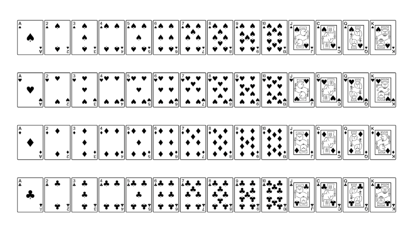
The Unicode values for the characters representing playing cards are laid out in a nice pattern. The last digit of the Unicode value corresponds to the point value of the card (aces low), and the second-to-last digit corresponds to the suite.

The ace of spades has code point U+1F0A1, and the aces of hearts, diamonds, and clubs have values  U+1F0B1, U+1F0C1, and U+1F0D1 respectively. The three of spades is U+1F0A3 and the seven of hearts is U+1F0B7.

But there’s a surprise if you’re only away of the standard 52-card deck: there’s a knight between the jack and the queen. The Unicode values for jacks end in B (Bhex = 11ten) as you’d expect, but queens end in D and kings end in E. The cards ending in C are knights, cards that don’t exist in the standard 52-card deck.

Here’s a little Python code that illustrates the Unicode layout.

for i in range(4):
   for j in range(14):
     print(chr(0x1f0a1+j+16*i), end='')
   print()

The output is too small to read as plain text, but here’s a screen shot from running the code above in a terminal with a huge font.

Unicode cards

Playing cards have their origin in tarot cards, which are commonly associated with the occult. But John C. Wright argues that tarot cards were based on Christian iconography before they became associated with the occult.

What can JWST see?

The other day I ran across this photo of Saturn’s moon Titan taken by the James Webb Space Telescope (JWST).

If JWST can see Titan with this kind of resolution, how well could it see Pluto or other planets? In this post I’ll do some back-of-the-envelope calculations, only considering the apparent size of objects, ignoring other factors such as how bright an object is.

The apparent size of an object of radius r at a distance d is proportional to (r/d)². [1]

Of course the JWST isn’t located on Earth, but JWST is close to Earth relative to the distance to Titan.

Titan is about 1.4 × 10¹² meters from here, and has a radius of about 2.6 × 10⁶ m. Pluto is about 6 × 10¹² m away, and has a radius of 1.2 × 10⁶ m. So the apparent size of Pluto would be around 90 times smaller than the apparent size of Titan. Based on only the factors considered here, JWST could take a decent photo of Pluto, but it would be lower resolution than the photo of Titan above, and far lower resolution than the photos taken by New Horizons.

Could JWST photograph an exoplanet? There are two confirmed exoplanets are orbiting Proxima Centauri 4 × 10¹⁶ m away. The larger of these has a mass slightly larger than Earth, and presumably has a radius about equal to that of Earth, 6 × 10⁶ m. Its apparent size would be 150 million times smaller than Titan.

So no, it would not be possible for JWST to photograph an expolanet.


[1] In case the apparent size calculation feels like a rabbit out of a hat, here’s a quick derivation. Imagine looking out on sphere of radius d. This sphere has area 4πd². A distant planet takes up πr² area on this sphere, 0.25(r/d)² of your total field of vision.

Fizz buzz walk

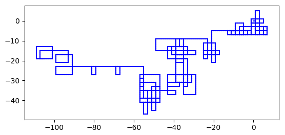
I ran across a graphic yesterday made by taking a sequence of steps of the same length, turning left on the nth step if n is prime, and otherwise continuing in the same direction.

Here’s my recreation of the first 1000 steps:

You can see that in general it makes a lot of turns at first and then turns less often as the density of primes thins out.

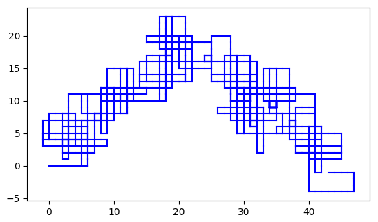
I wondered what the analogous walk would look like for Fizz Buzz. There are several variations on Fizz Buzz, and the one that produced the most interesting visualization was to turn left when a number either is divisible by 7 or contains the digit 7.

Here’s what that looks like:

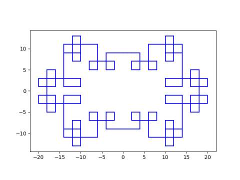
I wrote about something similar four years ago using a different rule for turning. That post looks at a walk on the complex numbers, turning left when you land on a Gaussian prime, a generalization of primes for complex numbers. These images have more symmetry and form closed loops. For example, here’s the walk you get starting at 3 + 5i.

starting at 3 + 5i

The starting point matters. See the earlier post for more examples with different starting points.

Related posts